Smartphone Imaging Technology and its Applications

Background: Evolution of the mobile phone imaging syetem for the mass consumer market

From mobile phone to smartphone

Smartphone today

Tomorrow’s smartphones

Mobile Imaging

Market development

Supply chain

Background: Brief history and milestones of smartphone imaging technology

Physical prroperties and requirements of smartphone photography

Camera form factor and image sensor size

• Smartphone flat housing 7-10 mm thick $\rightarrow$ cell phone optic $< 5-6$ mm
• Relative flatness factor: $r = \frac{L}{\Theta_{im}}$
  • $L$: overall length
  • $\Theta_{im}$: still feasible full image diagonal
• “The image sensor should be as large as possible so that as much light as possible falls on a pixel. This reduces fundamental disadvantages such as image noise, a reduced by dynamic range or longer exposure times and thus motion blur.”
• Factor $r$ depends on the field of view of the lens and its layout (standard upright, periscopic, etc.)
• Wide-angle lenses: $r=0.83$ (iPhone 6, an image diagonal $\Theta_{im}$ of 6 mm, an overall length $L$ of 5 mm)
• Thicker or a slightly protruding camera housing and complex 7-lens designs: $r = 0.65$ (an image diagonal $\Theta_{im} > 12$ mm)
• Image sensor sizes of the main camera (standard wide-angle) are integrated into several high-end smartphone models.

Image sensor resolution

• Standard image resolution of 12 megapixels
• Aspect ratio (square format adjustable for both landscape and portrait format)
  • SPC: 4:3
  • Full-format/APS-C: 3:2
• Image sensor formats (“inch values”)
  • $\Theta_{im}=$ 6 mm (width 4.8 mm, height 3.6 mm) $\leftrightarrow$ 1/3
  • Inch specification was taken from old Vidicon video tubes from 1950s and corresponded to the outer glass diameter of the photoelectric front surface.
  • The sensor diagonal corresponds to about 2/3 of the inch value. (Misleading! $\rightarrow$ dimensions in mm better!) <img src="/images/Vidicon_camera_tube.png" alt=“drawing” width=“50%”/>
• Why 12 MP in 1 $\mu m$ pixel pitch era
  • Keeping the same image sensor size (~6 mm), the pixel pitch reduced from about 6 $\mu m$ down to 1 $\mu m$.
  • Pixel amounts far greater than 12 MP are not beneficial due to practically unused resolution.
  • Consequences of reversed pixel race: reasonable amount of image data, better image noise, and better dynamic range
  • SPC image sensors with high number of pixels are not made up of adjacent Bayer patternsm but rather “multicell sensors” (Tetracell by Samsung, Quad-Bayer by Sony, 4-Cell by OmniVision)
    • Enhance light sensitivity (but similar can be achieved by using larger pixels)
    • Flexivility: can be read out in various ways (by selecting different sensitivities/exposure time , the dynamic range can be increased, or noise can be reduced through pixel binning, or output with very hgih-resolution image)
    • Pixels available when recording and pixels used to display the images
• Why 12 MP when 0.7 $\mu m$ pixel pitch by 2020
  • Additional cameras of different focal lengths can achieve the disired resolution of 8 or 12 MP in standard Bayer Pattern.
  • The multi-cell sensors mastering since smaller pixel pitch is challenging in mass production.
  • 12 MP still good in terms of the physiological limits of the human eye. (at best no more than 2000 x 1000 pixels are required for 6.2’ display)
  • Significant more pixels are necessary for enlargement or VR “under a magnifying glass”

Optical resolution and required aperture

• Definitions:
  • Airy dist (airy diffraction disk) : “When light passes through any size aperture (every lens has a finite aperture), diffraction occurs. The resulting diffraction pattern, a bright region in the center, together with a series of concentric rings of decreasing intensity around it, is called the Airy disk”
  • Point spread function (PSF): impulse response (function) of a focused optical imaging system. The Fourier transform of it is optical transfer function (OTF) of an imaging system.
  • Relative encircled energy $= 0.73$: a significant portion of the light distribution inside a square-shaped pixel.
  • Effective encircled brightness $> 0.8$: the intensity transferred to a grey value distribution by the photo conversion curve and opto-electronic conversion fucntion.
  • Modulation transfer function (MTF): measure contrast as part of image quality evaluation
• Diameter of the airy disk of the ideal image is $d_{airy} = 2.44 \lambda \frac{f}{d_{pupil}}$, where $\lambda$ is the wavelength and $f$ is focal length, $\frac{f}{d_{pupil}}$ is f-number (e.g. f-number is 1.4, written as f/1.4)
• An appropriate relationship between the diameter of the airy spot and the sensor pixel pitch $p$: $d_{airy} = 2 \cdot p$
• Set the corresponding critical f-number as: $\frac{f}{d_{pupil}} = \frac{p}{1.22\cdot\lambda}$, which for 6 mm image sensor and $p = 1.2\mu m$, is $1.8$ (or written as f/1.8)
• Telephoto lenses (normal focal lengths and short/long portrait focal lengths) with f-stops of $2.4$ or more and smaller pixels (e.g. $p = 0.8\mu m$)
• Nyquist frequency: $f_{Nyq} = \frac{1}{2p}$
  • Depending on the exact position relative to the pixel grid, a vastly differing contrast can be created.$\rightarrow$ specify image quality starting at $~f_{Nyq}/2$.
  • The system constrast is often displayed simultaneously with different fine structure periods (for $p = 1.2\mu m$, $f_{Nyq}/8$ = 52 lp/mm, $f_{Nyq}/4$ = 104 lp/mm)
  • Optics MTF * Sensor MTF has an increasingly statistical character near $f_{Nyq}$ due to relative position dependence with pixel grid
  • Moir$\acute{e}$: briefringent structured filters are expensive; point spread function of SPC lens is already larger, has a low-pass effect
• A limited spatial frequency for ideal incoherent optical system: $\nu_{max} = \frac{1}{\lambda f_{f-number}}$, unit is lp/mm.
  • $MTF_{ideal}(\nu) = \frac{1}{\pi}[acrcos(\frac{\nu}{\nu_{max}}) - \frac{\nu}{\nu_{max}\sqrt{1-(\frac{\nu}{\nu_{max}})^{2}}}]$ for $\nu\leq2\nu_{max}$
  • Monotonous, almost linear for large spatial frquencies
  • The same figure for SPC also for full-frame cameras
  • SPCs are physically limited by their size alone. $\leftrightarrow$ diffraction-limited.
• Abberation is so small that stopping down (f stopping down) would lead to a weaker contrast
  • SPCs have no iris diaphragms
  • Exposure is adjusted solely via the exposure time and the ISO sensitivity via the read-out AD amplififer on image sensor.
  • For full-frame, maximum contrast is obtained at around f/4, f/5.6, or f/8 before stopping down to the diffraction limit.
  • Loss of contrast with an open aperture is due to the fact: larger aberrations are allowed for simpler, compact design.
• Resolution is not independent from SNR of the image sensor

Portrait photography: perspective, bokeh, and depth of field

• Wide-angle lens: full diagonal field of view: $tan(FOV/2) = \frac{\Theta_{im, ff}/2}{f}\rightarrow FOV = 2arctan(\Theta_{im, ff}/(2f))$
  • ff: full-format
  • $f$: focal length (e.g. 35 mm, 28 mm)
  • The full image diagonal for a classic standard wide-angle lens (“allrounder lens”) of 35 mm: $\Theta_{im, ff} = \sqrt{36^{2} + 24^{2}} = 43.3$ mm
  • $FOV \approx 75\deg$ for $f = 28$ mm
  • Equivalent SPC focal length: $f = f_{eq}\frac{\Theta_{im, SPC}}{\Theta_{im, ff}} = 3.9$ mm
• Close-up portrait (face almost fills the vertical image field)
  • The distance from entrance pupil to the object: $\frac{s}{y_{ob}} = \frac{f}{y_{im, SPC}} \rightarrow s \approx 400$ mm, where $2y_{im}$ is the total length of the side of the vertical (short direction).
  • 40 cm is a typical distance at which one holds a smartphone (selfies, video calls etc.). So, an equivalent focal length of 28 mm is suitable as a front camera.
  • Typical normal portrait distances with a vertical side length of 0.72 m are about twice as large (i.e. 0.8 m). To have people completely in the picture, $y_{ob} = 2.16$ m (i.e. 2.4 m).
  • Wide-angle lenses are not well suited for portraits: $f_{eq} = 28$ mm and $s = 0.4$ m. The nose will be 10-20 % of the object distance in front of the ears, so it is imaged magnified and leads to deformations on the face.
  • Classic portrait focal lengths: equivalent focal length $f_{eq} \approx 85$ mm, which is 3 times longer.
• DSLR
  • The person is detached from background due to shallow depth of field
  • Defocused point spread function is larger with a longer focal length $\rightarrow$ spot diameter of the light source in the background with the same f-number and the same image format scales approximately in the ratio of the focal lengths.
  • SPC lenses have large depth of field. /
• Calculation of the size of the point spread in the depth and from the depth of field
  • Definitions
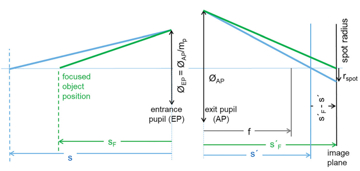
    • $s$ and $s’$ are for out-of-focus, $s_{F}$ and $s_{F}’$ are for focused.
    • Pupil magnification: $m_{p} = \frac{\Theta_{AP}}{\Theta_{EP}}$, typically [0.5, 1]
    • $\Theta_{AP}$: exti pupil, $\Theta_{EP}$: entrance pupil
    • $K$ is f-number (e.g. 1.8, 2.2)
    • Numerical aperture: $NA’ = \frac{1}{2K}$
    • Etendue: a property of light in an optical system, which characterizes how “spread out” the light in area and angle
  • By comparing trianlges, the ratio of the radius of the defocused point image $r_{spot}$ to the position of the defocus in the image space $(s’-s_{F}’)$: $\frac{r_{spot}}{|s’ - s_{F}’|} = \frac{\Theta_{AP}/2}{s_{F}’} = \frac{1}{2K} \rightarrow r_{spot} = \frac{|s’ - s_{F}’|}{2K}$
  • Focusing conditions: $\frac{1}{f_{ob}} + \frac{1}{f_{im}} = \frac{1}{f} \rightarrow -\frac{1}{m_{p}s} + \frac{m_{p}}{s’} = \frac{1}{f}$ and $-\frac{1}{m_{p}s_{F}} + \frac{m_{p}}{s_{F}’} = \frac{1}{f}$
  • By substitution, $r_{spot} = frac{f^{2}}{2K}\frac{|s - s_{F}|}{(f/m_{p} + s)(f/m_{p}+ s_{F})}$
  • With $f/m_{f} \approx 0$, the diameter of the image’s circle of confusion: $\Theta_{spot} = 2r_{spot} = \frac{f^{2}}{K}\frac{|s_{F}-s|}{s_{F}s}$
  • For easier comparing the imaging lenses with different image formats, relative circle of confusion: $\Theta_{rel.spot} = \frac{\Theta_{spot}}{\Theta_{im}}$, directly indicates the spot size ion the defocused area as it appears in the photo
  • For a infinitely distant background, $\Theta_{rel.spot, \inf} = \lim_{s\rightarrow\inf}\frac{f^{2}}{\Theta_{im}Ks_{F}}$
  • With definition of f-number: $K = \frac{f}{\Theta_{EP}}$ and magnification $m = \frac{\Theta_{im}}{\Theta_{ob, Portrait}} \approx \frac{f}{s_{F}}$, $\Theta_{rel.spot, \inf} = \frac{\Theta_{EP}}{\Theta_{im}}m$
  • For approximate object distance 700 mm: $\Theta_{rel.spot, \inf} = \frac{\Theta_{EP}}{700 \text{ mm}}$
  • $\Theta_{EP, ff} = \frac{f}{K} = \frac{135\text{ mm}}{2} = 67.5 \text{ mm}$, $\Theta_{rel, spot, ff} \approx 10%$; $\Theta_{EP, SPC} = \frac{f}{K} = \frac{4\text{ mm}}{2} = 2.3 \text{ mm}$, $\Theta_{rel, spot, SPC} \approx 0.3%$
  • With $\tan(FOV/2) = \frac{\Theta_{im}/2}{f}$, $\Theta_{rel.spot, \inf} = \frac{\Theta_{im}NA’}{700\text{ mm}\cdot\tan(FOV/2)}$. With a given FOV, the relative diameter of the circle of confusion is directly proportional to the product of image field diameter and the numerical aperture of the image.
  • Optical systems Etendue (“throughput”/“collecting power”/“A$\Omega$ product”): $G = \frac{\pi}{4}\Theta_{im}^{2}NA’^{2} \rightarrow $\Theta_{rel.spot, \inf} = \frac{\sqrt{G}}{700\text{ mm}\cdot \tan{FOV/2}}\rightarrow \Theta_{rel.spot, \inf}\propto\sqrt{G}\rightarrow$ 7x smaller image diameter and 7x larger NA’ achieve the same background circle of confusion. But not feasible for high-aperture lenses (SPC lens)
  • Depth-of-field: threshold the size of the circle of confusion $\Theta_{thres} = \Theta_{im}/1500$.
  • Hyperfocal distance: $s_{F, hyp} = \frac{f^{2}}{K\Theta_{thres}} + f \rightarrow \frac{f}{2K\tan{FOV/2}/1500} + f$. The image is shape from $s_{F, hyp}/2$ to infinity.
  • Autofocus is only required for close range.
  • SPC “portrait mode” achieved with depth and/or high-resolution 3D sensors

$\acute{E}$ tendue and photographic exposure

• Exposure controlled by ISO (sensitivity of the image sensor), exposure time, and amount of light described by $\acute{E}$tendue $H\propto ISO\times (\frac{1}{K})^{2}\times T$
• SPC does not have iris diaphragms for controlling aperture size
• ISO
  • Sensitivity of the image sensor $\rightarrow$ depends on the area of a pixel (pixel pitch size) $\leftarrow$ No. of photons strike each time
  • Efficency for a pixel absorbs light and converts into an electrical voltage
  • No. of photon per pixel is inversely proportional to $c^{2}$, where $c$ is crop factor. Crop factor (format factor/focal length multiplier) $c$ of an image sensor format is the ratio of the dimensions of a camera’s imaging area compared to a reference formrat, usually 35 mm format (full-frame)
  • $c = 7\rightarrow$ 49 times fewer photons. This corresponds to 5-6 exposure values ($EV = \log_{2}(K^{2}/T)$). $\rightarrow$ issues in low light and/or with fast-moving objects
  • High level of sensitivity $\rightarrow$ short exposure time and increased image noise
• Sunny 16 rule
  • On a sunny day with an ISO 100 film and f/16, the required exposure time is about 0.01 second
  • E.g. increase 3 f-stops in aperture to f/5.6 $\rightarrow$ 8 times shorter exposure (1/800 second) or ISO of 50 and 1/400 s
• Long exposure times cause issues in shaking hand in still photographs $\rightarrow$ reduced in SPC through optical and electronical image stabilization
• Image sensor technology (“binning”, “deep trench isolation”, “dual conversion gain”, “higher quantum efficiency”)
  • Binning: squares of pixels are binned into larger pixels. Artificially increase pixel size, gather more signal, flexibility of a camera sensor
    • CCD/EMCCD sensor is binned on the sensor before readout, meaning that it occurs before read noise is introduced by converting photoeletrons into grey levels. improving SNR and increased frame rate.
    • CMOS sensor is binned off the sensor after readout, meanning that read noise has been introduced to each pixel. Combining a 2x2 section of pixels together results in double the read noise for resulting super-pixel. 4 times signal 2 times read noise $\rightarrow 2:1$ boost in SNR, no speed benefits. However, CMOS camera is already far faster than CCD/EMCCD.
    • CMOS Binning. 3 noise sources: photon shot noise ($\sqrt{s}$), read noise (a fixed value for the sensor), and dark current; Noise are adding in quadrature ($\sqrt{\sum{n^{2}}}$)
  • Deep trench isolation: suppress electrical crosstalk; a DTI sidewalls passivation step is needed to avoid any degradation on dark current and white pixel number due to additional interface degects caused by DTI etch
  • Dual conversion gain licensed by Sony: 2 readout modes: one that includes a capacitor in the path, to provide extra electron storage capacity for bright, high DR conditions; the other that disengages this capacitor, delivers less dynamic range but increases the conversion gain, boosting the signal for low light conditions; before readout noise introduced
  • Higher quantum efficiency (QE): measure of effectiveness of an imaging device to convert incident photons into electrons (95% means sensor exposed to 100 photons producing 95 electrons of signal, from 95% to 20% varies by photons wavelengths)
    • Blue response is reduced due to front surface recombination. Front surface passivation (fabrication prrocess) affects carriers generated near the surface, and since blue light is absorbed very close to the surface.
    • Green response is reduced causing by reflection and a low diffusion length. Green light is absorbed in the bulk of a solar cell and a low diffusion length will affect the collection probability from the solar cell bulk and then reduce the QE in the green protion.
    • Red response is reduced due to rear surface recombination, reduced absorption at long wavelengths and low diffusion lengths.

David versus Goliath: the pros and cons of miniaturization

• Crop factor
  • $c = \frac{\Theta_{im, ff}}{\Theta_{im, SPC}} = \frac{43.3\text{ mm}}{\Theta_{im, SPC}}$, $c = 3.5$ to $12$
  • Depends on SPC sensor size, and lens FOV
  • With the assumption of containing equal number of pixels (12 MP), pixel pitch is larger by $c$ for full-format sensor
  • Further assumptions of same f-number $K$ and same FOV, $\bar{f} = f/c$, $\bar{\Theta_{im}} = \Theta_{im}/c$, $\bar{L} = L/c$ are scaled inversely with crop factor; Entendue/throughput and sensor area are scaled by $/c^{2}$.
  • Advantages
    • Geometrical scaling including weight and volume reduction
    • Optical distance (can focus on much smaller subjects)
    • depth-of-field scales linearly with focal length $f$ meaning that the hyperfocal distance $s_{F, hyp}$ is a factor of $c$ further away from the miniature lens. This increases image quality (less focusing errors). However, not capable for creating an artistic shallow depth of field.
  • Disadvantages
    • sees much less ligiht ($1/c^{2}$ since pixel area reduction, either $c^{2}$ larger exposure time or ISO, large ISO introducing more noise by $c$; $H~ISO\times (1/K^{2})\times T$)
    • Not capable for shallow depth of field
• Lens aberrations
  • Ray aberration spot scaled down by $1/c$ and pixel pitch scaled down by $1/c$
  • Airy spot size (diameter of airy diffraction disk, $\Theta_{airy} = 2.44\lambda K$; diffration point spread function) stays the same
  • Though ray aberration spot stays the same relative to the scale of pixel, the resolution is dropped linearly by $1/c$ due to the diffraction-limited lens design.
  • Lohmann’s scaling law, the spot area $A_{p}’ = \lambda^{2} K^{2} + (1/c)^{2}\bar{\epsilon^{2}}$, where $\bar{\epsilon^{2}}$ is the second moment of the ray deviation distribution.
• Multi-camera systems containing many thin lenses in parallel.
  • Increase effective image sensor area
  • Combining the images of various cameras to improve the image performance in various directions (e.g. noise reduction, HDR)
  • Stereographic 3D depth

SPC lenses: quality evaluation

• A common choice of spatial frequencies for MTF evaluations at full format is 10, 20, and 40 lp/mm, which are corresponding to $Nyq/8$, $Nyq/4$, $Nyq/2$ for full-frame format camera pixel pitch size $p = 6.25\text{ } \mu m$, respectively ($Nyq = 1000/2p$ lp/mm, $p$ in $\mu m$)
• MTF at original size (ff/8) is only slightly maller compared to the upscaled version of the lens $\rightarrow$ upscaled SPC to full-frame is comparable with excellent full format lenses
• According to the Lohmann’s scaling law, at t he original size with respect to imaging with smaller pixel pitch is moly moderately limited by diffraction compared to the aberration level of the lens design.
• When the lens size is scaled down the overall performance severely drops. The diffraction contribution in Lohmann’s scaling law becomes dominant.
  • Strehl ratio ([0,1]): evaluate lens performance in comparison to the diffraction limit. Strehl ratio $\uparrow$, diffraction limited $\uparrow$
  • Performance is pirncipally limited for yet smaller lens sizes
  • Predominantly diffrection-limited
• Makes little sense to achieve pixel resolutions far below $0.7-0.8\mu m$, which is the current state of the art for image sensor CMOS technology

The multicamera system in modern smartphones

• Standard wide-angle camera as main camera: 28 mm, FOV 75$\deg$
• Multicamera system for rear: a main camera, a shorter focal length with FOV of 120$\deg$, a longer focal length (55 mm or 70 m or 125 mm), a 3D depth sensor (based on ToF measurement) for a real-time depth maps of a scene
• Multicamera system for front: standard wide-angle lens + larger camera with a high-resolution image sensor (multicell for HDR) and autofocus, 3D sensing camera for face recognition (next to the visual cameras)
• Diagonal field of view, equivalent focal length, sensor size, sensor pixel number, pixel pitch, f-number, focal length, MOD (minimum optical distance), depth of field, image stabilisation

Optical system design

Optical design structure of a smartphone

• Criteria
  • Substracting the housing and image sensor thickness, the overall length of the lens must not be longer than about 5-6 mm
  • The image sensor should be as large as possible for reducing the disadvantages of a small image sensors (noise, dynamic range, see less photon)
  • The aperture ofoo the lens must be relatively large, about f/2 or larger, so that the system resolution is not limited with image pixel sizes
• Relative flatness factor $r = \frac{L}{\Theta_{im}} \approx 0.65 \cdots 0.85$; Despite the highly miniaturized desing, the crop factor is around $4$ away frorm ff image sensors
• Why plastic asperical lens for SPCs
  • No sperical lens type has large aperture of around f/2 and a small length-to-image-diameter ratio at the same time.
  • Asperical lens for SPCs are shorter in length and better in performance:
    • Higher contrast and lower peripheral light intensity drop (both due to lack of vignetting)
    • Both distortion and chromatic aberrations are comparably very good
• Plastic spherical lens$\rightarrow$ Plastic aspherical lens; FOVs around $60\deg$ and $75\deg\rightarrow$ $20\deg-150\deg$
• As pixel shrinking: Doublets/triplets$\rightarrow$ 4 lenses$\rightarrow$ 7 lenses and more; f-number decreased
• The optical design of SPC lenses is rarely dealt with in the literature
• Comparisons between Biogon lens and SPC lens
  • Biogon lens
    • Negative outer lens + positive inner lens group
    • Negtive outer element: chiefray is bent to a smaller angle inside the lens $\rightarrow$ smaller aberration contributions; off-axis entrance pupil becomes larger, improving illumination
    • Asymmetrical aberrations including distortion, coma, and lateral chromatic are elimiated by the quasi-symmetric arrangement around the stop in the center of the system. They get cancelled. <img src="/images/chromatic_aberration.png" alt=“drawing” width=“50%”/>
    • Longitudinal and high-order chromatic aberrations are corrected by low-dispersion glasses for the outer negative lens and the achromats of the inner positive lens
    • Spherical aberration and astigmatism are remainning to be corrected by fine-tunning all lens parameters.
    • Astigmatism: one where rays that propagate in two perpendicularr planes have different foci.
  • SPC lens
    • Both have field of view about $80\deg$
    • Ray angle at the entrance of the lens $\approx$ at the lens exit
    • Half of the system structure to the image plane is sufficient: aberrations (in particular distortion and coma) are corrected by the aspheres.
    • With the strong aspherical design, the digital correction would bring almost no advantage.
• Wide-angle lenses for SLR cameras are forced to use a retrofocus type becuase of the space required for folding mirrow between the last lens and the image sensor
• Modern lenses for mirrorless cameras are increasingly asymmetrical.
• Correction distortion, curvature, and astigmatism $\rightarrow$ aspherical lenses are placed directly in front of the image plane
• SPC lens
  • High-order awberrations are used here to reduce low-order aberrations
  • All lens surfaces are aspherical
  • Standard surface description of aspheres: $z = \frac{xrr^{2}}{1 + \sqrt{1-(1+k)c^{2}r^{2}}} + a_{4}R^{4} + a_{6}r^{6}+ \cdots$, where $c$ denotes the curvature at the apex of the surface, $k$ denotes the conical constant and $r$ denotes the radial distance from the optical axis.
    • The first term: different conic shapes: $k = 0$, sphere; $-1<k<0$, ellipsoid with main axis on the optical axis; $k = -1$, paraboloid; $k < -1$, hyperboloid
    • Typical asphere for SPC: w-shaped lens
    • The low aberration orders are largely compensated for with high-order aspheres, but residual high-order aberrations remain
  • The pupil and the field must be sampled sufficiently
  • SPC optics must hardly have any vignetting by lens edges or aprtures $\rightarrow$ reducing the aperture and loss of resolution towards the image corners
  • Mobile wide-angle lenses
    • The geometric light path to the corner of the image is more than 20% langer than it is to the center of the image
    • The numerical aperture size remains the same up to the edge of the image $\rightarrow$ keep the diffraction-limited resolution almost constant up to the corner of the image $\rightarrow$ change the refractive power depending on the image field height $\rightarrow$ w-shaped last lens (refractive power at edge: positive, center: negative; varies over the field height) $\rightarrow$ aperture at the field edge » conventional spherical optic
    • Characteristic of standard wide-angle lenses: chief rays strike the image plane at a simiarly high angle as they enter the lens ($\pm 35\deg-40\deg$)
    • For standard wide-angle lense, the chief ray runs along a line through the lens; for telephoto and extreme wide-angle types, chief ray has a global bending $\rightarrow$ standard wide-angle lenses are the most compact lens type among SPC lenses; image sensor used for standard wide-angle lens iat he largest within the multicamera systme

Optical design imaging performance

• Optical image performance evaluation of camera lens design: MTF (vs. FOV, spatial frequencies, distance to the image plane), distortion (radial distortion, TV distortion, and distortion grid plot), relative illumination, aberrration (spot diagrams, ray aberration curves, chromatic focus and lateral shift), angle of incidence at image sensor
• MTF vs. spacial frequencies up to the cut-off frequency ($1/(\lambda K)$)
  • Image performance of all lenses if diffraction-limited near the image center and drops off
  • The through-focus region with very high contrast is roughly only about $\pm 10 \mu m$ for all lenses
• Distortion graph
  • Not noticeable (<1%)
  • Barreldistortion of the extreme wide-angle lens is about 20%, which is not corrected by software as well $\rightarrow$ perspective distortion
• Relative illumination
  • Drops more towards toe corner of the image field for wide-angle lenses (“shading”). This is corrected by software and cause an in crease noise sensitivity by 1 or 2 EV ofr wide-angle photography
  • Includes a natural geometrical loss according to approxinmately $\cos^{4}{angle-of-incidence}=\cos^{4}{35\deg}\approx 0.45$
• Angle-of-incidence graph shows the chief ray and marginal ray angles in the image plane
  • Avoiding light loss, the chief ray incidence angle is limited to $<35\def$
  • The oblique incidence on the image sensor results in further intensity losses (included in the software-corrected shading) $\leftarrow$ improved by back-side-illuminated image sensors, specific architexture (e.g. deep-trench structures), and slightly shifting the micro lenses according to the incidence angle
• Ray aberration on the tangential and sagittal image plane for different wavelengths versus field
  • Averration curves are very “wiggly” as residual aberrations of the compensation principle of low-order aberrations by high-order aberrations through usage of high-order aspherical lens surface deformations
  • Chromatic aberrations can be physically evaluated (image simulations of edge or line spread functions vs. field and through focus; “color fringe widths”)

Extreme wide-angle lenses

• Short flatness factor $r = L/\Theta_{im}<1$; with additional negative “bending lens” at the front, $r$ is even larger
• Beam path is comparable with standard wide-angle lens; chief ray angles $\approx 35 \deg$ on the image plane
• Optical desings of extreme wide-angle lenses with an even larger FOV of up to around $150\deg$ and $160\deg$ with ~50% distortion

Tele lenses

• Smaller image sensors and smaller apertures
• Difficulties of compact telephoto lenses: longer $f$, samller the required telefactor($TF = L/f$)
  • TF<1: refractive power is positive in the front part and lens and negative in the rrear; The smaller TF more positive orr negative refractive power required, then leads to greater lens curvaturres and larger aberrations
  • Optical performance is severely limited as the $f\uparrow$

Periscope tele lenses and alternative tele concepts

• Periscope layout: with $45\deg$ mirror or with $45\deg$ prism mirror
  • Mirror size and entrance pupil size < depth of the housing
  • $f\uparrow\rightarrow K\uparrow\rightarrow$ the diffraction limited resolution weaker
  • e.g. $\Theta_{EP} = 4$ mm, relative small aperture of $f/3.4$, $f = K\cdot\Theta_{EP}=13.2$ mm
• Entrance pupil can be made rectangular with a larger f-number in the long direction
• Catadioptric layout: 2 mirrors in the front or with several reflections between the mirrors ($TF<0.5$)
  • Allows a very large entrance pupil diameter $\rightarrow$ high aperture ratio
  • Aperture ratios can reach to f/1 with large cetral obscuration $\rightarrow$ distinct loss of contrast in the lower spatial frequencies $\rightarrow$ fine structures would be displayed with a higher contrast (irrelevant to SP dimensions, this high resolution cannot be used due to the available pixel sizes)
  • Pors: loss of contrast; “donut bokeh” bused by obscuration (i.e. ring-shaped out-of-focus highlights)

Zoom

• Very good optical zoom systems for compact digital system cameras (DSC) also integrated in mobile phone
• Digital zoom was also available very early on cell phones
• Since 2016, standard: hybrid zooms through multi-camera systems using lenses of different focal lengths

Hybrid zoom in multicamera systems

• The combination of different fixed focal lengths in modern SP multicamera systems
• The achievable optical resolution of SPC lenses is heavily dependent on the specific optical design, in turns depends on an equivalent $f$.
  • Assuming a diffraction-limited optical resolution of $res_optics = 0.5\cdot \Theta_{airy} = 1.22\cdot\lambda\cdot K$
  • All these resolved area on the image sensor surface (4:3 aspect ratio) $A_{im} = \pi\cdot(\Theta_{im}/2)^{2}\cdot 0.48 = \pi/4\cdot0.48\cdot\Theta_{im}^{2}$
  • The number of “optical pixels” (i.e. resolved areas, optical resolution ) $NP_{optics} = \frac{A_{im}}{\frac{\pi}{4}res_{optics}^{2}}\approx 0.32\frac{\Theta_{im}^{2}}{\lambda^{2}K^{2}}$
• Simplified consideration for digital zoom and the image sensorr resolution to estimate the total resolution of a hybrid multi-camera zoom system over the entire focal length range: $NP_{\text{optics digital zoomed}} = NP_{potics, 0}\frac{f_{0}^{2}}{f^{2}}$, where index 0 corresponding to lens index 0
  • Digital zoom reduces the resolution according to the cropped FOV, whcih is directly scales with $f$
  • For image sensor that has 4-pixel of a Quad-Bayer sensor structure $NP_{sensor} = \frac{NP_{sensor, total}}{NP_{macro-pixel}}$, $NP_{macro-pixel} = 1$ for standard Bayer sensor and $NP_{macro-pixel} = 4\text{ or }{9}$ for 2x2 or 3x3 multi-cell sensor.
• A well-balanced system should have about the same resolution of optics and image sensor
  • Roughly the case for extreme wide-angle and standard tele camera lenses
  • For main camera, the optical resolution is clearly bettern than the image sensor resolution. Sensor limits the overall resolution
  • For periscopic long tele camera, the image sensor limits the overall resolution
  • Optical performance of wide-angle lens > tele and periscope tele lenses even at the same effective focal length when zoomed in digitally
  • The actual resolution of the complete wide-angle camera system < tele cameras, since the digitally zoomed-in pixel resolution is worse for $f_{eq}>56$ mm
  • $NP_{effective} = min(NP_{optics digital zoomed}, NP_{sensor})$
• Improve image performance with image fusion in the common FOV of both cameras
  • Simulate of all steps in camera ISP and the specific algorithm how images are fused by multiple cameras
  • Requires joined camera module calibration
  • Hard at close range due to the parallax of the images caused by the spacing of the camera modules

Optical zoom systems

• A classical optical zoom changes the imaged object frame (i.e. FOV) by changing $f$ of the system $\rightarrow$ changing the distance between the lens between the lens elements
• Two optical groups with $f_{1}$ and $f_{2}$: $\frac{1}{f} = \frac{1}{f_{1}} + \frac{1}{f_{1}} - \frac{d}{f_{1}f_{2}}$
• For SP, the realized image performance of an optical zoom system can decrease significantly at long focal lengths; The image sharpness drops due to the diffraction limitation
• For DSC, excellent image performance can be achieved with relatively loose space constraints
  • Digital-optical co-optimization
  • A significant portion of lens elements are aspherical
  • Digital aberration corrections are made (wid-angle range, a distortion of approx 20-30%) $\rightarrow$ image is cropped somewhat depending on the zoom
  • Zooms with a large zoom factor, the aperture in the long focal length area is reduced to limit the diameter in the front area and the overall length
  • Can reach to 20x or 50x which SPCs unachievable

Opto-mechanical layout and manufacturing

Plastic lenses: Key miniature opto-mechanical layout

• Pros:
  • Distinctly aspherical lens shape
  • Key to the small depth of SPC optics
  • High complexity of the structural shapes
  • Possible to implemnt and mechanical mount
  • Accuracy in the sub-$\mu m$ ranges
• Special noncontact interferometric measurement technology for measuring small, complex components at steep angles of incidence
• Contact-mode measurement devices for measure component shapes

Opto-mechanical layout

• No measurements during assumbly process. MTF measurements are carried out once assembly is complete
• Improve quality, individual lens elements are matched to another from the injection molding cavities.
• The lens elements are positioned directly on top of each other on the flat plastic mountint rings (the ring stops to prevent straylight)
• SPC lenses: high accuracy, sensitive to decentering or tilting
• Plastic lenses manufacturing by injection/pression into precise molds while still in liquid form; not stable as glass; manufactured after about 1 minute
• Plastic lenses cons: relatively low refractive indices with a large dispersion $\rightarrow$ mitigated in the future with nano composites
• Limitations
  • No cemented lense like for glass lenses
  • Thermal sensitivity $\rightarrow$ refractive index and expansion coeffcient $\rightarrow$ aberration type: focus shift $\rightarrow$ compensated by autofocus

Active optical assembly

• The lenses are aligned with the image sensor and glued in with UV adhesive; Automatically in a few second
• During the assembly process on the sensor, the barrel is aligned in the degrees of freedom
  • centering x/y, tilt x/y and focus distance until the specified spatial frequency response (SFR) values are reached simultaneously over the image field
  • The MTF values is monitored over long periods of time
• In 6 axes, the optical axis between camera modules

Tolerancing and yield analysis

• Set permitted deviations from the theorertically achievable image performance
• Inspection process:
  • During the production processm, the quality of the optics is qualified on the basis of MTF values during the final inspection done by the optics module supplier for the system integrator. (not yet connected to image sensor)
  • The system integrrator adjusts the optics to the image sensor so that the final image performance of the SPC qualified with SFR measurements.
  • SFR is the common notation of the MTF of the complete system optics/sensor
• Yield analyses (reject analyses)
  • Done in the final stages of optical design with Monte Carlo analyses
  • The optical desingers use their own sensitivity analyses to set tolerances for the lens (radius, thickness, aspherical deviations, deviations in the regractive index, dispersion of the plastic) and their relative positioning errors in assembly (decentering, tilting, spacing deviations, etc.) and probability distributions of individual errors.
  • “Rolls” many different systems
  • MTF data for these systems gives a statistical distribution $\rightarrow$ system MTF specification

Wafer-level Manufacturing

• Low-cost; thin
• Micro-electromechanical systems (MEMS)-based sensors (e.g. gyroscope, accelerrometer), photonic chips (photonic integrated circuits (PICs))

Anti-reflection coating for plastic lenses

• Important in scenes with a large dynamic range, especially with bright light sources (residual light reflections straylight or “ghosts” on the image plane)
• Reflections on optical surfaces $\leftarrow$ destructive interference from a single or multilayer coating by properly choosing layer thicknesses and material refractive index
  • Camera lenses have AR coatings with multilayer coating of 2 or 3 materials of thicknesses of about 10 to a few 100 nm
  • Coating process cannot easily transferred to glass (adhesion, lower melting temp, etc.)
  • A uniform coating thickness is difficult $\rightarrow$ atomic layer deposition (ALD)

Image sensor

• A CMOS sensor is a matrix of semiconductor photodiodes that detects the irradiance distribution on the sensor surface.
  • According to the irradiance distribution on the sensor chip and the exposure time ($T$), electrons are generated as charge carriers in the individual photodiodes and converted by capacitors, a voltage is finally generated. Then, A to D.
  • Each individual photodiode is provided with its own electronic circuit: readout amplifier read out individually at each XY coordinates
  • A higher bit value in AD converter does not necessarily lead to better image quality; image quality depends on noise behavior of the image sensor and image motif
  • Only portion of the cell surface is sensitive to light due to wiring
  • Microlens covers the the entire sensor for collecting as much of the incident light as possible and avoiding shadowing within the cell structure
  • The voltage level ($\rightarrow$ image signal) on the individual photodiodes depend solely on the respective brightness and the exposure time ($T$)
  • Color filter array (Bayer pattern, RGGB) $\rightarrow$ de-Bayering/demosaicing; The color cameras with a Bayer mask have a lower resolution thanmonochrome cameras $\rightarrow$ some SPC multicamera systems equiped with monochrome camera modules for high-resolution image and color information from second camera
  • DSLR with mechanical shutter $\rightarrow$ almost simultaneous exposure; SPC with purely electronically exposure control, exposure is done during readout $\rightarrow$ individual photodiodes are not exposed and readout at the same time $\rightarrow$ runtime effects i.e. rolling shutters limiting in slow motion mode; electrronic “global shutter” (Sony 2017)
  • Additional IR band pass filter to block residual significant portion of light in IR (silicon has a monotonically increasing sensitivity from blue towards IR); For 3D face or iris recognition, IR cut-off at e.g. 840 nm or 950 nm.
• OECF (Opto-Electronic Converrsion Function) response/characteristic curve
  • Horizontal axis: physical intensity of the light received by the image sensor; Irradiance (radiation power per area, $W/m^{2}$) or Luminous efficiency function (CIE standard, luminance intensity per area, $cd/m^{2}$); in linear scale or log scale
  • Vertical axis: digital numeric value (0-255 for 8 bits, 0 to 1000 for 10 bits)
• Photoconversion curve/camera response function
  • Horizontal axis: exposure value (EV, $EV = \log_{2}(k^{2}/T)$)
  • Vertical axis: no. of electrons ($\equiv$ digital numeric value)
  • Relation between the number of electrons and the luminance
  • Noise limit: minimum brightness on the pixel (minimum signal); signal rises from the noise limit; forr SPC CMOS sensors: 1-2 electrons
  • FWC (full well capacity): the capacity of the potential well of the diode; CMOS sensors: 4k - 5k electrons
  • 0 EV set at FWC or close to the saturation value $\rightarrow$ noise limit/value can be readout
  • Dynamic range: ratio of the maximum and minimum signal (e.g. here is $10$ EV)
• Quantum Efficiency (QE, $\eta$, [0,1]): the probability of whether a photon, which enters the sensor finally generates an electron in the photo-electric layer
  • Transmission (coating and material absoption)
  • Geometry of microlens and the entire light path
  • $\lambda$
  • Angle of incidence
  • Numerical aperture of the incident light
• Deep trench isolation: walls are built between the pixels enhancing the QE and reducing cross-talk
• Stacking technology: light sensitive rear illuminated photodiode array is separated from the electronics (back-side illuminated sensors, i.e. BSI, higher sensitivity due to shorter and undisturbed path)

Image processing

• Create the most natural image possible of the object; enhance in terms of contrast or color rendition
• Computational imaging
  • Combines several images from the same or different camera modules (3D sensors etc.)
  • Encoded or phase-distorted apertures can be deployed in combination with deconvolution (e.g. extend the depth of field i.e. EDoF)
  • 3D acquisition and image recognition; AR
• Pipeline: noise reduction, linearization, shading correction, white balancing; demosaicing, distortion correction, to sRGB, gamma correction, sharpening, jpeg compression (more details can be found $\rightarrow$ Course Notes/CS231m)
  • Photoconversion curve is fitted to an 8-bit brightness scale by a tone value curve
  • Greater sharpening to medium or low spatial frequencies (human are particularly responsive); Moderately on high-frequency areas (This limits for complex motifs for low-light shots)
  • Different tone value curves are generally used for different photographed scenes to optimize the image (contrast, brightness, color)

Noise and noise reduction

• Small pixels: more sensitive to light; lower SNR; lower FWC $\rightarrow$ smaller dynamic range
• SPCs compensated by image processing and sensor technology (e.g. deep trench isolation, binning, dual conversion gain, and higher quantum efficiency)
• Noise from electrons is minor in CIS (contact image sensor) in good lighting conditions; Photon noise dominates for all cameras
• Software-based noise reduction irrevocably smooth out small image details (i.e. resolution smaller, structures with less contrast $\rightarrow$ human skin appear unnatural)

Focusing

• Depth of field of SPC lenses is significantly greater than that of full-frame camera lenses
• Previous rule of thumb: for SPCs object distances of >1 m, no focusing is required
• For high-end standard wide-angle lens FOV = 75$\deg$, $\Theta_{im} = 12$ mm, $f = 7.82$ mm, f-number $K = 1.7$, then the hyperfocal distance is $4.5$ m. $\rightarrow$ if the lens is focused to an object distance of 4.5 m, the image is sharp for all object distances between 2.24 m to infinity
• Focusing range and accuracy – key parameters
  • Focusing accuracy: no. of depth rranges within the complete focusing range
  • 1st depth range: 2.25 m to infinity
  • 2nd depth range: 2.25 m set as far distance, calculate the lower limit of the depth range
    • $s_{F, hyp} = h = 4.5 = \frac{f^{2}}{Kr\Theta_{im}}$
    • Realtive PSF spot size for sharp resulting image: $r = 1/1500$
    • $s_{near} = \frac{s_{F}}{1+s_{F}/h}$
    • $s_{far} = \frac{s_{F}}{1-s_{F}/h}$
    • Index $j$: successive depth ranges; $s_{near, j} = s_{far, j+1}$, with $s_{F, 0} = h = 4.5$, so $s_{F, 1} = h/3$…$s_{F, j} = h/(2j + 1)$ for adjacent depth ranges
    • The depth range quickly decreases: $s_{F, 3} = 0.9$ m (-15 cm, +23 cm) to the foreground and background is still sharp
    • Focusing distance $s_{F, 23} = 0.1$ m (-22 $\mu$ m, +23 $\mu$ m)
    • Depth ranges in terms of magnification instead of $s_{F}$: $m_{F} = \frac{s_{F}’}{s_{F}} = \frac{f}{s_{F} + f}$ with $s_{F}»f \rightarrow m_{F}\approx \frac{f}{s_{F}}$
    • The depth range number $j$ linearly related to the magnification $m_{F} = (2j+1)\frac{f}{h}$
    • With minimum optical distance $s_{F, j} = s_{MOD} = h/(2j + 1)$, total number of depth ranges $J = \frac{h}{2S_{MOD}}$; SPC lens $J = \frac{4500mm}{2\cdot 100mm}\approx 23$
  • 3 focus steps per depth range $\rightarrow$ $3J\approx70$ focus postions; With total movement of lens actuator $\approx$ $0.28$ mm $\rightarrow$ positioning accuracy $0.28/70=4$ $\mu$ m $\rightarrow$ focusing accuracy $\Delta m_{F, acc}\approx \frac{f}{3h} = \frac{K}{2250\tan{(FOV/2)}}\approx 0.001$
  • Focusing accuracy depends on f-number $K$ and FOV according to the equation; also depend on actual size of the lens
• Front cameras: fixed focus, depth map cameras with a larger f-number providing greater depth of field
• Focusing: autofocus system, modification of the optical imaging system for movement, mechatronic implementation of the drive

Autofocus methods: Contrast and phase detection (more details can be found $\rightarrow$ Other Notes/3A)

• Phase detection on reflex cameras: “phase contrast measurement”; with a mirror attached to the beam splitter and a separate image sensor, the deviation from the focus is quantitatively determined using triangulation
  • Pros: acquire optimal focal point exactly from the target shift from a single measurement
  • Cons: need folding mirror between lens and image plane (required space, larger lenses)
• Contrast detection in digital age: in the read-out image, until contrast is at its maximum
  • Pros: compact design
  • Cons: slow, need multiple measurements; swing back and forth; “bad direction move”; error-prone or fails for low-contrast objects (especially low-light conditions)
• SPC Phase detection auto focus (PDAF)
  • contrast detection $\rightarrow$ phase contrast pixels $\rightarrow$ dual pixel AF
  • Phase contrast pixels: “light version” of SLR phase contrast; some masked pixels at 4 different orientations (5-10%) are used as focus pixels (not available as normal senosr pixels); left “blind spots” to be interpolated
  • Dual pixel AF
    • Under a common mirolens have two separate neighbored pixels (“photodiode twin”); does not suffer from blind spots
    • Towards outer field regions, PDAF becomes problematic due to the oblique incidence of light (35 $\deg$ in the image corners)
    • Cooptimization of pixel architecture, microlens design, and data processing can be supported by ray-tracing and wave-calculation-based image simulations
  • ToF or lidar for active distance measuring systems to improving spatial resolution
  • Taking a whole stack of pictures (“live image” or “motion still”), once the object is in focus, switch to high resolution, save the image, and delete the image stack from the buffer.

Optical system changes focus position

• Entire lens (“total lens focusing”) or partial individual optical groups (“floating element focusing”, adpoted for SPC)
• Deforming lens with liquid lenses (electrowetting); A pair of aspherical components that can be moved laterally
• Focusing distance: $-\frac{1}{s}+\frac{1}{s’} = \frac{1}{f}$, where $s$ is the object distance, $s’$ is the image distance from the front or rear principal plane
• The lens is moved forward in order to focus on an object that is closer to the lens
• The distance required for focusing scales almost quadratically with the focal length, not linear: $\Delta s’{MOD} = s’{MOD} - f = -\frac{f}{s_{MOD}+f}$
• Even with same f, but differently sized image sensors have different distances to move for focusing
• With magnification equation $m = \frac{s’}{s} = \frac{f}{s+f}$, the focus offset $\Delta s’_{MOD} = -mf$, $\rightarrow$ a lens with focal length f, the focus movement distance directly scales with magnification
• DSLR: the typical close distance magnification is about 1:10; SPC: a close distance of 100 mm magnification is about 1:15
• The longer focal lengths, more space is required for the focus movement
• Preferably with 2 moving groups to achieve sufficient image performance

Focusing mechanism: Voice coil motors (VCM) and other concepts

• VCMs
  • Almost exclusively used in SPCs as drives for the focus movement of the lens
  • Structure: AF VCM and housing attached on the image sensor plane, the outer case has folded connector cable and gimbal vois coils
  • Issues with predictability in its location ($10 \mu$ m) due to directional hysteresis (image depth of field, temperature, coil resistance variation) $\rightarrow$ open-loop control before correct focus
• Alternative actuator types: stepper motors, piezo motors, MEMS, EDoF
• EDoF (extended depth-of-focus) by computational imaging
  • 3rd order profile aspherical extends the DoF at the expense of contrast
  • Recovered by deconvolution with a priori data of the phase mask
  • 2 DoF extension, which in turn translates to a significant extension of DoF in object distance equal to minimum optical distance (MOD = 30 cm). Less than a standard AF with barrel shift (MOD $\approx 10$ cm)
  • Moving the lens to a desired focus position is obsolete
  • Cons: noise from decomvolution (especially in low-light condition, can cause unrecoverable contrast)

Image stabilization

• During image exposure, imageing performance limited by human hand-shaking, low light conditions, etc. due to intrinsically low etendue and a lower FWC $\rightarrow$ longer exposure ($\times$ squared crop factor, approx 50 for same f-number), ISO $\uparrow$ introducing additional noise
• The weight of SLR also helps reduce hand shaking
• Electronic image stabilization (EIS) and optical image stabilization (OIS) used simultaneously
  • Front cameras may not contain OIS
  • EIS: Hand shaking as measured with on-board gyroscope and accelerometer; image frame is slightly cropped and conpensated by frame shift
  • EIS cons
    • Cannot help in movement during one-frame exposure, would result in blur $\rightarrow$ can be reduced by deconvolution of the intergral PSF (computationally intensive task)
    • Limited to FOV portion since working on reduction of FOV $\rightarrow$ larger hand-shaking amplitudes result in residual errors
  • OIS: residual aberrations since the degrees of freedom used in the OIS system are not the same (pitch, yaw, roll)

Hand-shaking and image blur

• Human tremor: involuntary oscillatory movement of body parts directly caused by muscles contracting and relaxing repetitively
• The key for EIS and OIS is the availability of on-board MEMS-based (micro-electro mechanical systems, gyroscope, accelerometer, etc.) miniature sensors.
• With differential capacities in comb-drive actuator design, the sensitivities of the sensors are linear and high-voltage sensitivity, leading to low power consumption
• 6 degree of freedom: 3 transitions (x, y, z), 3 angular directions (pitch, yaw, roll) denoted $\theta_{x}$, $\theta_{y}$, $\theta_{z}$
  • Image point $(x’, y’)$, object point $(x, y)$
  • $dx’ = f’d\theta_{y} + \frac{f’}{s}dx + yd\theta_{z}$
  • $dy’ = f’d\theta_{x} + \frac{f’}{s}dy + xd\theta_{z}$
  • 1st components: pitch and yaw, measured by gyroscope
  • 2nd components: measured by accelerometer
  • 3rd components: roll (azimuthal-oriented blur, increases linearly in a radial direction from the image center)
  • $\theta_{x}$, $\theta_{y}$, $\theta_{z}$ are simliar in amplitude $\rightarrow$ the roll-induced blur in the image corner is purely geometrically related to the yaw and pitch induced blur offsets (e.g. $\tan{(FOV/2)} = \Theta_{im}/(2f’)$, lens with FOV of $\75\deg$ has a factor of about 0.75 smaller blur in the image corner compared to yaw and pitch induced blur)
• Most OIS systems are not able to compensate for this component (“usual” situation is < $1\deg$; most OIS is $0.5$-$1\deg$)
• “Normal” object distances (e.g. 1m), angular dominates; close-distance, decenter components dominate; at about $0.3$ m the contributions are comparable
• Typical hand-shaking blur is not a purely random walk, containing some systematic components
• SPCs interior images: exposure time 1/10 s; night scenes: 1 s; image blur is in the order of 10 pixels

Optical image stabilization implementations

• OIS systems: barrel decenter (most common); image sensor decenter (in SLR referred to as body image stabilization BIS); gimbal
• In a first-order approximationd a tilt and shift of the barrel is equvalent $\rightarrow$ correction of a hand-shaking tilt or decenter
• Barrel decenter: compensating movement of the entire lens barrel in x, y with a voice coil motor; some systems, barrel is tilted
  • Stiffness of the springs: correctable amplitude frequency distribution (e.g. very stiff spring $\rightarrow$ high-freq corrections but smaller amplitudes at low freq)
  • Yoke: tight adjustment incresases friction and hysteresis; loose adjustment may lead to parasitic tilts
• Image sensor decenter: iPhone 12 Pro, image sensor is actively moved
• Gimbal syetem: vivo X51,tilts the complete barrel together with the fixed-to-barrel image sensor

Dynamic range

HDR imaging

• The limited dynamic range of image sensors in relation to the range of irradiances in a scene
  • Typical outdoor scenes: 9-12 EV, rarely above 14 EV
  • Strong light source: > 20 EV
  • High-end, full-frame digital consumer cameras: DR $\approx$ 14-15 EV (DxO Mark)
  • SPCs: DR $\approx$ 10-12 EV (DxO Mark)
• DR as low ISO sensitivity: DR decreases as ISO increases (0.6-1.1 EV per ISO step, e.g. ISO 6400 DR 6-9)
• Calculate HDR images from a sequence of different exposoure times
• The tone values of these HDR recordings, which extend over a very large value range (e.g. 16 bits) are reduced to a much smaller brightness range (e.g. 8 bits)
• Scene recorded several times with different exposure times and combined for the extended dynamic range according to the brightness range shown
• Unsuitable for fast-moving subjects and more tend to loss of resolution due to hand shaking
• Mitigated with multicell sensors (exposure times of different lengths to be parallelized with different pixel clusters, with pixel binning)

Lens flare and ghosts

• When the sum or another very birght light source is in or just outside the frame, DR > 25 or 30 EV
• Lens quality is crucial: residual light reflection on lens surfaces from a bright light source may superpose or cover up parts of the image; even for multilayer coated surface (<0.2% reflectivity)
• Double reflex: with image sensor 5% reflectivity $\rightarrow$ 1/10000 weaker $\rightarrow$ -14 EV from the light source; but the maximum irradiance within normal scene is about 15 EV smaller than the light source
• No. of lens surface-surface reflections inside lens with $n$ surfaces: $n + (n - 1) + \cdot \cdot \cdot + 2 + 1 = \frac{1}{2}n(n + 1)$; all surfaces including in and between micro lens, IR filters, etc.
• Shapes: Caustics or crescent-shaped (large aperture); egg-shaped (smartphone); often purple (from higher coating reflectivity in blue and red)
• Every scene with a large dynamic range
• Good hardware (i.e. AR coatings, straylight-blocking rings), the straylight performance can be optimized on optical design phase to avoid in-focus ghosts (modifications on the optical surface shapes, opto-mechanical layout of the system)
• May appear inside a very small portion of the full FOV (distinct local differrences in reflection direction at the wiggly lens surfaces; surfaces exceeding the total reflection angle)
• Testing in the lab: local variation of straylight can easily be observed when rotating the lens relative to a very bright light surface

Portrait mode

• Subject recognition $\rightarrow$ portraits of people, portraits of pets, etc; context-by-context basis; shape of edges (face contours); combined with 3D acquisition to improve depth maps
• Computationally blurring out-of-focus regions according to the depth map data; depth dependent PSF stored in the memory; dependent on both depth and the selected focus to resemble the real images
• The depth map should accurately reproduce the scene in all its details
• The depth of field of an PSC is many times greater than that of the DSLR due to the much smaller image format
  • Relative size of the circle of confusion (diameter of the PSF): $\Theta_{rel, spot , \inf} = \frac{\Theta_{EP}}{\Theta_{ob, portrait}} = \frac{\Theta_{EP}}{700 mm}$
  • SPC equivalent focal length of 85 mm requires 85 mm / crop factor = 8.8 mm, resulting in entrance pupil diameter $\Theta_{EP} = 8.8 mm / 3 \approx 3 mm \rightarrow \Theta_{rel, spot , \inf} \approx 0.42%$
  • DSLR portrait lens with entrance pupil diameter of $85mm/1.4\approx 60mm$ and a relative background blur spot diameter of $\Theta_{rel, spot , \inf} \approx 8.7%$, which is 20 times larger for SPC

3D depth acquisition technology

• Can be deterrmined stereoscopically on the common image portion of the cameras
• Distance to objects can be determined for the directional component of the neighboring cameras and not in the direction perpendicular to it $\rightarrow$ with more cameras, the disparity can be captured along different directions, improves the quality of the depth map
• Multi-cameras: occluded area reduced, disparity more robust
• Classic multiview stereo processing is computationally expensive, challenging on mobile; involving feature extraction, feature matching, camera calibration and pose estimation, depth estimation, surface reconstruction, and texturing
• Lightfield imaging
  • Conventional lens is combined with a micro lens array with a much smaller focal length
  • Micro lens array is positioned closely in front of an image sensor
  • The raw image consists of many small partly overlapping fields of view of a scene
  • Correlation analysis between adjacent fields of view $\rightarrow$ dispartiy and depth
  • Smaller focal length results in small achievable disparities (<1%) and inferior higher depth resolution
  • Extended depth of field with different focal lengths
• Disparity calculation
  • Object points distances $s_{1}$, $s_{2}$; base distance between the cameras $b$; image positions $y_{1}$, $y_{2}$
  • $\frac{s_{1}}{b} = \frac{f}{y_{1}}$
  • $\frac{s_{2}}{b} = \frac{f}{y_{2}}$
  • Disparity $d = y_{2} - y_{1} = fb(\frac{1}{s_{2}} - \frac{1}{s_{1}})$
  • With $f = \frac{y_{max}}{\tan{(FOV/2)}}$, the disparity relative tot he image frame $\frac{d}{y_{max}} = \frac{b}{\tan{(FOV/2)}}(\frac{1}{s_{2}} - \frac{1}{s_{1}})$
  • Assume $s_{1}\rightarrow \inf$, $s = \frac{by_{max}}{d\tan{(FOV/2)}}$
  • $b$, $d$, $y_{max}$, FOV are known from lens, calibrated camera (positioning, axis-orientation)
  • Typical SPC $b$: 1-2 cm
  • For normal tele lens, a relative disparity of $d/y_{max} = 0.354$ (3.54% of the distance between image center and corner), which is about portrait distance for FOV $= 44\deg$; 2.5 m object distance, 20 pixels; 10 distance disparity, 2 pixels
  • Depth resolution decreases as distance from the lens increases
  • Depth resolution depends on the depth of field and actual focus position
  • For unstructured objects (e.g. clear blue sky), machine learning
  • Quality of the depth map highly dependent on the contrast and light intensity, spectral distribution of the illumination in the scene
• Incorrect depth data unnatural blurring at the edge between foreground and background
• Face recognition requires 3D depth data: structured light camera system, ToF sensors (time of flight, range imaging camera, lower power light source infrared light; LiDAR: laser beams)
  • Light source: VCSEL (vertical cavity surface-emitting laser) at a power of ~150mW in near IR light
  • Modulated light for deduce temporally pulsed or continuous waved

Simulation of lens bokeh: Camera 3D point spread function

• Equation of the diameter of the geometrical PSF (“circle of confusion”): $\Theta_{rel, spot} = \frac{f^{2}}{\Theta_{im}K}\frac{|S_{F} - s|}{s_{F}s}$ for “normal imaing” without considering macro distances $\rightarrow$ when object distance $s < s_{F}$, $s\uparrow$, circle of confusion $\Theta_{rel, spot}\downarrow$; Further move the object, $s\uparrow$, circle of confusion $\Theta_{rel, spot}\uparrow$
• Bokeh (暈け/ボケ)
  • Non-uniform intensity distribution within an out-of-focus hightlight source is due to lens aberrations
    • Overlapping out-of-focus highlights
    • “Cat’s-eye bokeh” due to vignetting usually for high-aperture lenses (lens’ field stops in the front and rear part of camera lenses)
    • “Edgy bokeh” due to iris stop (diaphragm with blades)
    • Softar bokeh (softar filter scatters light out of nominal light path)
    • “Donut bokeh” (spherical aberration, red color fringe due to chromatic aberration) due to overcorrected low-order spherical aberration (redistribution of intensity in the presence of aberrations)
    • “Christmax ball bokeh” (spherical aberration)
    • “Fine structured bokeh” including “onion ring bokeh” (optical manufacturing induced residual surface deformations)
  • light intensity: not a problem when not exceeding DR; exceeding DR, irradiance is physically redistributed inversely proportional to the surface area of the out-of-focus spot $\rightarrow$ synthetic bokeh of an SPC spot brigihtness must be guessed

Portrait look: a quality evaluation

• Synthetic bokeh: depth map quality, inferior low-light, reduced DR
• Challenging in low-light: noisy face due to the low ambient light; unpleasant differences between artifitial smoothed background and noisy face; overexposed bright colored highlight on the background loss its DR appearing white $\rightarrow$ computed blurred background incorrectly displayed as white (unexpected larger defocusing area with less intensity than saturation value of the DR, not uniform, failed bokeh)
• DxO computational bokeh test setup
  • Critical objects for high-resolution depth acquisition in topologically enclosed areas like holes or tiny eyelets
  • Structured stipes which are placed diagonally into the depth for checking natrually and continuously sharpness transition in the depth
• Criteria based on the ideal of the natural bokeh
  • Depth map quality:
    • Subject background segmentation
    • Repeatability
    • Blur gradient smoothness (also 3D DSF model)
  • 3D PSF model
    • Bokeh shape
    • Equivalent aperture
  • “Noise” uniformity: Noise consistency (face noise and background smoothness)

Image performance specification and test

Lab evaluation during R&D; qualification in mass production (mentioned in 8.3, active optical assembly); qualification of the image quality, including signal and image processing in the SP

Lab evaluation during R&D: Objectively checking measurable optical and sensor properties

• Tests and standardized test charts
  • Resolution and contrast: CIPAA resolution (wedge) test chart, OECF/noise chart with 20 gray patches
  • Color reproduction: X-Rite color checker digital SG
  • Field of view (FOV) and distortion: 19/14-grid test chart
  • Dynamic range
  • Auto exposure (AE)
  • Autofocus (AF)
  • Auto white balance (AWB)
  • Lens shading
  • Color shading
  • Flare: Flare target, round dots forming a cross
  • Ghosts
• Other tests and inspections: material tests, dust and environmental tests, shock and vibration, continuous run, lifetime, electromagnetic compatibility, electronic tests (software and sensor interfaces to the camera, drives for VCM and OIS)

Evaluation of image quality in the imaging pipeline

• Subjective quality tests: test motifs including natural objects, special image arrangements, and people
• As objective as possible: trained person according to precisely specified test and evaluation procedures (lighting, viewing time, etc.)
• Image processing software takes place practically until the device is sold $\rightarrow$ assess as early as possible
• No recognized stantards forr the overall evaluation of a camera system
• DxOMark (broad public perception, commercial), VCX (nonprofit, consortium)

Smartphone camera interface with telescopes, microscopes, and accessory lenses

Summary and outlook

References:

1. Walasek-Hoehne, B., K. Hoehne, and R. Singh. “Video Cameras used in Beam Instrumentation–an Overview.” arXiv preprint arXiv:2005.04977 (2020).
2. https://www.edmundoptics.com/knowledge-center/application-notes/imaging/limitations-on-resolution-and-contrast-the-airy-disk/
3. Kapłonek, Wojciech, et al. “Optical profilometer with confocal chromatic sensor for high-accuracy 3D measurements of the uncirculated and circulated coins.” Journal of Mechanical and Energy Engineering 2 (2018).
4. https://www.photometrics.com/learn/camera-basics/binning
5. Tournier, A., et al. “Pixel-to-pixel isolation by deep trench technology: application to CMOS image sensor.” Proc. Int. image sensor workshop. 2011.
6. https://www.dpreview.com/articles/1570070253/what-is-dual-gain-and-how-does-it-work
7. https://www.photometrics.com/learn/imaging-topics/quantum-efficiency
8. https://www.pveducation.org/pvcdrom/solar-cell-operation/quantum-efficiency
9. https://optcorp.com/blogs/telescopes-101/the-basic-telescope-types