Stanford CS 231m

Panoramas

Can be achieved with wide-angle optics or rotation cameras.

System Overview

• Camera Module -> Video Frames -> Real-Time Tracking -> Camera Module
• Camera Module -> Images -> Warping -> Registration -> Blending -> Final Panorama

Cylindrical Panoramas

• Project each image onto a cylinder
• A cylindrical image is a rectangular array
• View: reproject a portion of the cylinder onto a picture plane representing the display screen
• Narrow FOV -> less distortion
• Same center of projection.

Stitching

Detect key points -> find corresponding pairs -> align images

Key Points

• Harris corner detector: $E(u,v) = \sum_{x, y}w(x,y)[I(x+u,y+v)-I(x,y)]^{2}\simeq\begin{bmatrix}u & v\end{bmatrix}M\begin{bmatrix}u \\ v\end{bmatrix}$, where $w(x,y)$ is window function ($1$ in window, $0$ outside or Gaussian)
• Measure of corner response: $M = \sum_{x,y}w(x,y)\begin{bmatrix} I_{x}^{2} & I_{x}I_{y} \\ I_{x}I_{y} & I_{y}^{2} \end{bmatrix}$
• Both $\lambda_{1}$ and $\lambda_{2}$ are not too large
• Another way with Haar instead of window function: $I_{x}$ and $I_{y}$ are x-oriented and y-oriented Haar filters at scale $\sigma$ and $M = \begin{bmatrix} \sum I_{x}^{2} & \sum I_{x}I_{y} \\ \sum I_{x}I_{y} & \sum I_{y}^{2} \end{bmatrix}$ over all the pixels in $5\sigma\times5\sigma$ neighborhood
• $R = det(M) - k(trace(M))^{2}$, $k \in [0.04,0.06]$, $R>0$ but not small
• Harris corner detector Workflow: corner response $R$ -> thresholding -> local maxima
• FAST (features from accelerated segment test) corners: look for a continuous arc of N pixels, all much darker/brighter than center pixel
  • Normally, radius is $3$, $N = 16$
  • For fast implementation: check pixel intensities of pixel $1$, $5$, $9$, and $13$ with the center pixel intensity. Then, check the rest of the $12$ pixels.
  • Limitations: when $N<12$, the detection rate is too high

Point Descriptors

Invariant and distinctive

• SIFT (Scale Invariant Feature Transform)
  • Locate high-variance interest points, representing them with a vector attribute of local gray level variations
  • DoG pyramid:
    1. 1 octave above the level before
    2. Each octave has images of same size
    3. Within octave, apply same Gaussian
    4. Downsample and upsample to restone resolution
  • Local extreme in DoG for each image ($D(x, y, \sigma)$)
    1. Local extreme among current and immediate recent $3x3x3$ pixels
       • It is recommended that finding the extrema for $>= 2$ different values of scale $\sigma$ in each octave
       • -> $>=4$ values for $\sigma$ -> At least 5 different scale Gaissuan images in each octave
    2. True locationn based on Taylor’s expansion: $\overrightarrow{x} = - H^{-1}(\overrightarrow{x_{0}})\cdot \overrightarrow{J}(\overrightarrow{x_{0}})$
    3. Threshold out the weak extrema: $|D(\overrightarrow{x})| < 0.03$
  • Dominant local orientation
    1. Gradient magnitude at local extreme location on Gaussian-smoothed image: $$m(x,y) = \sqrt{|ff(x+1,y,\sigma) - ff(x, y, \sigma)|^{2} + |ff(x, y + 1, \sigma) - ff(x, y, \sigma)|^{2}}$$
    2. Gradient orientation: $\theta(x,y) = \arctan \frac{ff(x, y + 1, \sigma) - ff(x,y,\sigma)}{ff(x+1, y, \sigma)-ff(x,y,\sigma)}$
    3. Weight $\theta(x,y)$ with $m(x,y)$
    4. Construct a histogram of $\theta(x,y)$ with 36 bins for 360 degree, the histogram peak/fitted parabola gives the dominant local orientation.
  • 128-dimentional vector
    1. Grdient magnitude is the same as previous step; Gradient directions are measured relative to the dominant local orientation
    2. At the scale of the extremum, the extreme point is surrounded by a $16\times16$ neighborhood of points ($4\times4$ cells, each cell contains $4\times4$ block of points). Magnitudes are weighted by a Gaussian where $\sigma$ is $1/2$ width of the neighborhood to reduce the importance of the points that are relatively far
    3. For each of the $16$ cells, and 8-bin orientation histogram is caluclated based on gradient-magnitude-weighted values of $\theta(x,y)$ at the $16$ pixels in the cell.
    4. Concat the $16$ 8-bin histograms yields a 128-element descriptor
    5. 128-element descriptor for each extremum in DoG -> normalized to unity for this 128 elements -> invariant to illumination
• Blob detection in 2D
  • Laplacian of Gaussian (LoG): Circularly symmetric operator for blob detection in 2D.
  • $\Delta^{2}_{norm}g =\sigma^{2}(\frac{\partial^{2}g}{\partial x^{2}}+\frac{\partial^{2}g}{\partial y^{2}})$, where $\frac{\partial^{2}g}{\partial x^{2}}=g(x-1, y)-2g(x,y)+g(x+1,y)$
  • Or with filter kernel $\begin{bmatrix}0&1&0\\ 1&-4&1\\ 0&1&0 \end{bmatrix}$
• SURF (Speeded Up Robust Features)
  • Interest point where determinant of Hessian is maximized (determinant of Hessian measures Guassian curvature of surface; Gaussian curvature$\uparrow$, strong variance in every direction)
  • Differences: integral images for fast caluclation of derivatives; only concept of pyramids; No downsampling; Resolution stays same
  • Integral images: $I(x,y) = \sum_{x}\sum_{y}f(i,j)$
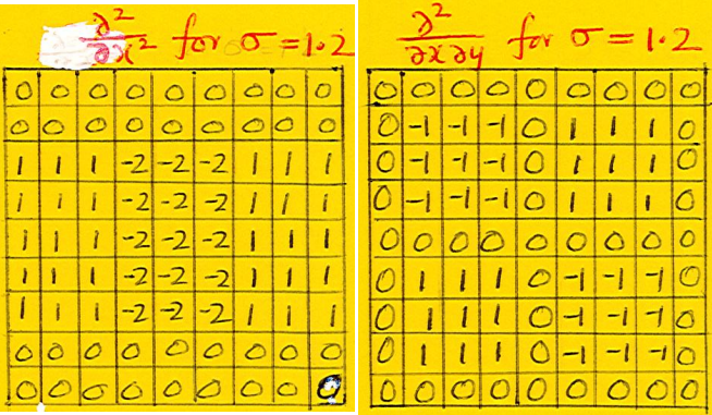
  • Discretization of $\frac{\partial^{2}}{\partial x^{2}}ff(x,y)$ in the Hessian
    1. Convolve the image $f(x,y)$ with $\frac{\partial^{2}g}{\partial x^{2}}$, where $g(x) = \frac{1}{\sqrt{2\pi}\sigma}e^{-\frac{x^{2}}{2\sigma^{2}}}$ -> actually, we need to convolve with half-width central lobe $h(x) = -\frac{1}{\sqrt{2\pi}\sigma^{3}}[1-\frac{x^{2}}{\sigma^{2}}]e^{-\frac{x^{2}}{2\sigma^{2}}}$
    2. Descrete 2D operators: The interest points are located at the pixels where the determinant is a maximum with respect $x$, $y$, and $\sigma$ /
    3. Calculate first-order derivatives $\frac{\partial}{\partial x}$ and $\frac{\partial}{\partial y}$ with Haar wavelet filters.
       • Basic forms of Haar wavelet: $\begin{bmatrix}-1 & 1\end{bmatrix}$ along $x$ and $\begin{bmatrix}-1 \\ 1\end{bmatrix}$ along $y$.
       • Scale up to $M\times M$ operator ($M$ is even; $M>4\sigma$)
       • Could use integral image $I(x,y)$
    4. Local dominant direction
       • Range: $6\sigma\times 6\sigma$ neighborhood
       • $(d_{x}, d_{y})$ are weighted with $2\sigma$-Gaussian centered at interest points
       • Scanning a scatter plot of the weighted $(d_{x}, d_{y})$ with a $60\deg$ cone. Largest resultant vector.
    5. Descriptor at scale $\sigma$
       • Range: $20\sigma\times 20\sigma$
       • Orientation: local dominant direction
       • $20\sigma\times 20\sigma$ neighborhood is divided into a pattern of $4\times4$ squares
       • Each squares (containing $5\sigma\times 5\sigma$ points) construct a $4$-vector $(\sum d_{x}’, \sum d_{x}’, \sum |d_{x}’|, \sum |d_{x}’|)$, where $d_{x}’$ and $d_{y}’$ are outputs of the two Haar operators relative to the lcoal dominant direction.
       • Total $64$-element descriptor vector at each interest point after concatnating $16$ $4$-vectors.
• ORB (Oriented FAST and Rotated BRIEF)
  • Use FAST-9 (Harris)
  • Find orientation: calculate weighted new center $\frac{\sum xI(x,y)}{\sum I(x,y)}, \frac{\sum yI(x,y)}{\sum I(x,y)}$
  • Reorient image so that gradients vary vertically
  • BRIEF (Binary Robust Independent Element Features): Gaussian smooth first; randomly choose a pair of pixels in a defined neighborhood around the key point (1st $\sigma$, 2nd $\sigma/2$); compare the pair of pixels intensities getting 1 or 0; Randomly choose pairs for $N$ times for $N$-bit vector; rotated BRIEF (rBRIEF) according to the patch orientation $R_{\theta}\times Q$, where $R$ is rotation matrix, and $Q$ is of shape $1\times N$
  • Feature matching: compare the binary vectors with Hamming distance(XOR + pop count)
• SuperPoint Self-Supervision Networks

Feature Matching

• SAD (Sum of Absolute Differences): $\min \sum\sum|f_{1}(i,j) - f_{2}(i,j)|$
• SSD (Sum of Squared Differences): $\min \sum\sum|f_{1}(i,j)-f_{2}(i,j)|^{2}$
• NCC (Nomalized Cross-Correlation): $\max \frac{\sum f_{1}(i,j)f_{2}(i,j)}{\sqrt{\sum f_{1}(i,j)^{2}\sum f_{2}(i,j)^{2}}}$

Aligning Images

• Homography = planar propjective transformation
  • Linear transformation on homogeneous $3$-vectors, the transformation being represented by a non-singular $3\times3$ matrix $H$
  • Point $x$: $x’ = Hx$
  • Line $l$: $l^{T}x_{i} = 0$ and $x_{i}’ = Hx_{i}\implies l’=H^{-T}l$
  • Conics $C$: $x^{T}Cx = 0$ and $x = H^{-1}x’\implies C’=H^{-T}CH^{-1}$
  • Maps a traight line to a straight line
  • Projective Group $\rightarrow$ Affine Group $\rightarrow$ Similarity Group $\rightarrow$ Euclidean Group
    1. $H = \begin{bmatrix} A & \vec{t}\\\vec{v^{T}} & \nu \end{bmatrix}$
    2. Affine: $\begin{bmatrix} 0&0&1 \end{bmatrix}$ for last row of $H$, keeps parallel lines parallel
    3. Similarity: $A^{T}A = \lambda^{2}I$ ($A$ is orthogonal), shpaes preserved
    4. Euclidean: $A^{T}A = I$ ($A$ is orthonormal), rigid body motion, preserve Euclidean distance
  • Affine transform maps $l_{\infty}$ to $l_{\infty}=\begin{bmatrix} 0&0&1 \end{bmatrix}^{T}$
  • General projective transform maps $l_{\infty}$ to vanishing line.
  • By sending vanishing line to $l_{\infty}$ can remove affine distortion.
• $x’ = Hx$ for each corresponding point pairs. Rearrange the equations. $\rightarrow Ah = 0$, where $A_{i} = \begin{bmatrix} -x&-y&-1&0&0&0&xx’&yx’&x’\\0&0&0&-x&-y&-1&xy’&yy’&y’\end{bmatrix}$. Decomposite $A$ with SVD. Solution is the nullspace of A, the last column/row of $V$/$V^{T}$. Or solve the least square problem of $min|Ah|$ with $|h| = 1$. Or set $h_{3,3} = 1$, solve least square problem of $|Ah-b|$ with solutioin of $h = (A^{T}A)^{-1}A^{T}b$
• RANSAC (Random Sample Consensus)
  1. Randomly choose a subset of data points to fit
  2. Within a threshold $\delta$ of model are consensus set (inliers). No. of inliers is $M$.
  3. Repeat for $N$ times. The model with biggest $M$ is the most robust fit
  • Assume $\epsilon = 10%$ outliers, goal: the probability $p$ for at least $1$ sample does not include any outliers For the case, $>1$ outliners included in current sample, the probability is $1-(1-\epsilon)^{n}$, where $n$ is no. of point pairs For $N$ samples, at least $1$ sample is free of outliers, the probaility is $1-p = [1-(1-\epsilon)^{n}]^{N}\rightarrow N = \log_{1-(1-\epsilon)^{n}}{(1-p)}$
• Hybrid Multi-Resolution Registration
  • Coarse-to-fine strategy: Pyramid from low resolution (downsampled) to high resolution (Upsampled)
  • Image based registration for initial guess
  • Feature based registration: feature detection (Harris corners) $\rightarrow$ feature matching $\rightarrow$ RANSAC$\rightarrow$ New estimate

Blending

Directly averaging the overlapped pixels results in ghosting artifacts (moving objects, errors in registration, parallax, etc.)

Alpha blending/feathering: $I_{blend} = \alpha I_{left} + (1-\alpha)I_{right}$

Issues

• Drifing
  • Vertical error accumulation <- Apply correction make zero sum in vertical displacement
  • Horizontal error accumulation <- Reuse 1st/last image for right panorama radius
• Ghosting
  • Assign one input image to each output pixel (graph cut)
  • Introducing new artifacts: inconsistency between pixels from images caused by exposure/white balance/vignetting
  • Poisson blending: copy gradient field from inputimage, reconstruct the final image with Poisson equation ($E = \sum s^{x}[I_{x}-g_{x}]^{2} + s^{y}[I_{y}-g_{y}]^{2} + wI^{2}$, where $g_{x}$ and $g_{y}$ is the target gradient values, $s^{x}$ and $s^{y}$ are smoothness weights, $w$ is panelized parameter for encourage/disencourage to go back to original pixel value) in the coarse multi-spline domain.
  • Laplacian pyramid blending:
    1. $L_{A}$ and $L_{B}$ are Laplacian pyramids of images $A$ and $B$. (Laplacian: Gaussian-expanded deeper level of Gaussian)
    2. Gaussian pyramid $G_{M}$ for selection mask $M$
    3. The combined pyramid $L_{S}$: $L_{S} = G_{M}\cdot L_{A}+(1-G_{M})\cdot L_{B}$
    4. Collapse the $L_{S}$ pyramid to get the final blended image.
  • Multi-resolution fusion: two images with different exposure time, use Guassian pyramid as weight matrix weight Laplacian pyramid to get a fused Laplacian pyramid to get a final image.
  • Two-band blening: high freq and low freq.

HDR Imaging

Dynamic Range

• Luminance: a photometric measure of the luminuous intensity per unit area of light travelling in a given direction (unit: candela per square metre $cd/m^{2} = lux$) * Eye can adapt from $10^{-6}$ to $10^{8} cd/m^{2}$ * without adaptation from $1$ to $10^{4} cd/m^{2}$ * with non-specular reflectance from $1$ to $10^{3} cd/m^{2}$ * Display: $1$ to $100 cd/m^{2}$ (0-255)

HDR Previous Methods

• Human HDR: sensitive to contrast (log scale); pupil; neural & chemical; transmition to brain
• Multiple exposure photography: map segments of high dynamic range to low contrasts
• Camera response curve calibration for the multiple images with various exposure time: adjust radiance to obtain a smooth response curve
• Dodging and burning: hide partial during exposure; exposure more to a region; smooth circular motions & blurry mask avoid artifacts
• Gamma correction
• Global tone mapping (various contrast for each image)
• Local tone mapping (Reinhard operator to avoid high light satrurated)
• Hitogram adjustment: lum not even $\rightarrow$ equalization, histogram in log space $\rightarrow$ issue: expand comtrast $\rightarrow$ trimming large bins (adjustment)
• Oppenheim: low contrast on low-freq, keep high-freq $\rightarrow$ issue: halo $\rightarrow$ bilateral filtering on intensity
• Exposure fusion: weights over 3 maps: Laplacian filter $\rightarrow$ contrast map; saturation on RGB respectively; exposure stretched based on gaussian distribution
• Multi-resolution fusion: Laplacian pyramid $*$ Gaussian Pyramid generate fused pyramid
• HDR video: auto exposure, motion compensation (registration between frames), tone mapping

System Overview

Reference frame selection $\rightarrow$ consistency detection $\rightarrow$ HDR generation $\rightarrow$ Poisson blending

HDR optical system

• Beam splitting prism breaks up the light into three parts, one for each sensor fitted with different filters
• With 2 beam splitters instead of prism to increase the light efficiency

Camera ISP

Pinhole Camera

• Without pinhole, all the sensor points would record similar colors (integral of light from every point on subject)
• Effect of pinhole size: large pinhole (geometric blur), optimal pinhole (too little light), small pinhole (diffraction blur)
• Lens
  • Gauss’s ray diagram
  • Focus distance: $\frac{1}{s_{o}}+\frac{1}{s_{i}} = \frac{1}{f}$
  • At $s_{o} = s_{i} = 2f$, get $1:1$ imaging
  • Depth of field: the range of distances that area in focus (can’t focus on obejcts closer to the lens than $f$)
  • Chromatic aberration
    • Different wavelengths refract at different rates $\rightarrow$ different focal lengths
    • To align red and blue with achromatic doublet: Crown lens (strong positive lens) + Flint lens (weak negative lens)
  • Lens distortion
    • Radial change in magnification: pincushion （corners stretching out）, barrel distortion (corners squeezing in)
    • Vignetting
      • Irradiance: radiant flux received by a surface per unit area. (Unit: $W\cdot m^{-2}$)
      • Radiant flux or radiant power: the radiant energy emitted, reflected, transmitted, or received per unit time * Irradiance is proportional to projected area of aperture as seen from pixel of image plane
      • Irradiance is proportional to projected area of pixel as seen from aperture
      • Irradiance is proportional to the distance^2 from aperture to pixel
      • Each of above factor $\approx \cos \theta$. Thus, light drops as $cos^{4}\theta$, $\theta$ is the angle measured from center of the aperture to the pixel versus horizontal line
      • Flat fielding: take a photo of a uniformly white object; resulting image shows attenuation

CMOS Sensor

• Structures
  • Front-illuminated sensor: on-chip microlens $\rightarrow$ color filter $\rightarrow$ metal wiring $\rightarrow$ light receiving surface $\rightarrow$ Silicon substrate, photo-diode and potential well
  • Back-illuminated sensor: on-chip microlens $\rightarrow$ color filter $\rightarrow$ light receiving surface $\rightarrow$ Silicon substrate, photo-diode and potential well $\rightarrow$ metal wiring
  • Metal wiring includes: transistors (amplifier, row select bus, column bus, reset)
  • Anti-aliasing filter: 2 layers of birefrigent material to split one ray into 4 rays (birefrigence: a refractive index that depends on the polarization and propagation direction of light)
  • Front-illuminated sensor: similar to eyes
  • Back-illuminated sensor:
    • Cons: Cross talk or color mixing with adjacent pixels; silicon waffer fragile
    • Pros: Increase light; captured improve low-light performance
• RAW
  • Pixel non-uniformity
    • Each pixel in a CCD has a slightly different sensitivity to light (within 1% to 2%)
    • Can be calibrated wiith a flat-field image
    • When calibrating with a flat-field image, the effects of vignetting eliminate as well as other optical variations
  • Stuck pixels: some pixels are turned always on or off $\rightarrow$ identify, replace with filtered values
  • Black level substraction: temperature adds noise; sensors usually have a ring of covered pixels around the pixels that exposed to source to capture the noise floor, subtract their signal
• AD Conversion
  • Sensor converts analog light signal to analog electrical signal
  • AD Conversion: $\geq10$ bits (often $12$ or more); linear response; No. of bits = No. of op-amp
  • Op-amp: $V_{out} = A\cdot(V_{in})$; Note that for op-amp, $V_{in,+}\approx V_{in,-}$
  • ISO = amplification in AD conversion
    • Before AD conversion, the signal can be amplified
    • ISO 100 means no amplification; ISO 1600 means 16 amplification
    • $+$ can see details in dark areas better
    • $-$ noise is amplified as well; sensor more likely to saturate
• Color Filter Array: Bayer Pattern
  • $\begin{bmatrix} \color{blue}B& \color{green}G& \color{blue}B&\color{green}G \\ \color{green}G&\color{red}R&\color{green}G&\color{red}R \\\color{blue}B&\color{green}G&\color{blue}B&\color{green}G \end{bmatrix}$
  • $36$ megapixels contain $9$ megapixels of R, $18$ megapixels of G, and $9$ megapixels of B.
  • Demosaicking: separate RGB into 3 channels
    • Bilinear interpolation: easy to implement; fails at sharp edges
    • Dealing with edges: bilateral filtering
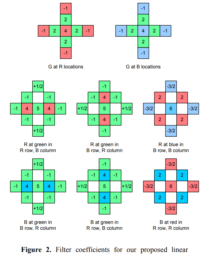
    • Dealing with edges: compare the red value to its estimate from the bilinear interpolation with the nearest 4 read pixels; add a proportion of this difference to the interpolation results for green value estimation at the location. The difference indicates change of luminance. $\hat{g}(i,j) = \hat{g}(i,j) + \alpha \Delta_{\hat{R}}(i,j)$
  • Denoising using non-local means
    • Image self-similarity can be used to eliminate noise: average a group of squares which are almost indistinguishable
    • BM3D (Block Matching 3D)

Color Science (More Details can be found → Course Notes/Purdue ECE 638)

• CIE Chromaticity Diagram
  • Intensity is imeasured as the distance from origin black $(0,0,0)$
  • Chromaticiity coordinates given a notion of color independent of brightness
  • $x+y+z=1$ yields a chromaticity value dependent on dominant wavelength (hue) and excitation purity (saturation, distance from equal energy white point $(1/3,1/3,1/3)$)
  • Perceptural non-uniformity: the XYZ color space is not perceptually uniform (MacAdam ellipse, just noticeable difference)
• CIE L*a*b* uniform color space
  • Approximate human vision, L component closely matches human perception of lightness
  • a channel: red-green; b channel: blue-yellow
• YUV, YC_bC_r, …
  • Family of color spaces for video encoding
  • Eye is sensitive to luminance $\rightarrow$ separate luminance and chrominance
  • Get low frequency UV compressed; Filters color down (2:1, 4:1)
  • Channels: Y = luminance (linear); Y’ = luma (gamma corrected); UV/C_bC_r = chrominance (always linear)
  • Y’C_bC_r is not an absolute color space (the actual color depends on the RGB primaries used)
  • YC_bC_r is YUV represented differently
    • YUV: luminance and BR luminance
    • YC_bC_r (scaled YUV): luminance, blue minus luminance (B-Y), and red minus luminance (R-Y)
    • YP_bP_r (physical YC_bC_r): analog version of YC_bC_r, physical component video cable used to transmit YC_bC_r
• Gamma encoding
• Luminance from RGB
  • Green will appear the brightest, red will appear less bright, blue will be the darkest
  • For luminance by NTSE, CIE, ITU are different for RGB gain
• Cameras use sRGB
  • standard RGB color space (uses the same primaries as used in studio monitors and HDTV, gamma curve typical of CRTs, direct display)
  • Need a map from sensor RGB to sRGB, need calibration
• Linear or non-linear
  • linear: simulatinmg physical world
  • non-linear: HVS, minimizing perceptual errors due to quantization
• Film response curve (Density vs. Log exposure)
  • Toe region: chemical process
  • Middle linear region: a given amount of light turned half of the grain crystals to silver, the same amount more turns half of the rest
  • Shoulder region: close to saturation
  • Toe and shoulder preserve more dynamic range at dark and bright areas at the cost of reduced contrast
  • Film has more dynamic range than print (~12 bits)
• Digital camera response curve(Intensity vs. irradiance)
  • Irradiance: radiant flux received by a surface per unit area
  • Use different response curves at different exposures

3A (More Details can be found → Other Notes/3A)

• Auto focus
  • Filter pixels with configuragle IIR filters (infinite impulse response) to produce a low-resolution sharpness map of the image
  • The sharpness map helps estimate the best lens position by summing the sharpness values (=focus value) either over the entire image or over a rectangular area. (coarse to fine strategy)
• Auto white balance
  • Illuminant determines the color normally associated with white by HVS
  • RAW image has more green color
  • Identify the illuminant color $\rightarrow$ neutralize the color of the illuminant
    • Prior knowledge of illuminant color temperature
    • Known reference object in the picture: find some white or gray
    • Gray world assumption (gray in sRGB space)
  • Methods
    • Grey card (a picture of a white or grey obejct, deduct the weight of each channel)
    • An object with known $(r_{w},g_{w},b_{w})$
    • Use brightest pixels that is not saturated/clipped, make it white
  • Mapping the colors
    • For a given sensor: pre-compute the transformation matrices between the sensor color space and sRGB at different temperatures
    • For an unknown sensor: interpolating between pre-computed matrices
  • Estimating color temperature
    • Use gray world assumption (make average of all pixels gray $R=G=B$) in sRGB space (just using $R=B$)
    • Estimate color temperature in a given image
      1. Apply pre-computed matrix to get sRGB for $T_{1}$ and $T_{2}$
      2. Calculate the average values $R$, $B$
      3. Solve $\alpha$
• Auto exposure
  • Parameters: exposure time, aperture, analog and digital gain, ND (nertral density) filters (modifies intensites without change in hue)
  • Exposure metering: CDF of image intensity values, $P$ percentile of image pixels have an intensity lower than intensity $Y$; Separate highlights and shadows areas

Image Formatting

• JPEG encoding
  1. RGB $\rightarrow$ YUV/YIQ and subsample color
  2. DCT (discrete cosine transform) on $8\times8$ blocks
  3. Quantization
  4. Zig-zag ordering and run-length encoding
  5. Entropy coding
  • Notes: Quantization tables and entropy coding tables are stored in between header and image data
• Other formats:
  • JPEG2000: ISO = $2000$; better compression, inherently hierachical, random access; much more complex
  • JPEG XR: Microsoft 2006; ISO/ITU-T, 2010; good compression, supports tiling (randomly access without having to decode whole image); better color accuracy (including HDR); transparency; compressed domain editing

Camera APIs

• Traditional camera APIs
  • Real image sensors are pipelined: while one frame exposing, next frame is being prepared and previous frame is being read out.
  • Viewfinding/video mode: pipelined, high frame rate; settings changes take effect someime later
  • Still capture mode: paramteres prepared; reset pipeline between shots
  • Image sensor: (exposure, frame rate) configure $\rightarrow$ expose $\rightarrow$ (gain, digital zoom) readout
  • Imaging pipeline: (format) receive $\rightarrow$ (Coefficients) Demosaic $\rightarrow$ (white balance) color corr
• The FCam Architecture
  • A software architecture for programmable cameras: expose the maximum device capabilities
  • Image sensor
    • no global state
    • state travels in the requests through pipeline
    • all parameters packed into requests from application processor
    • at expose stage takes charge of lens, flash, etc. of the devices; The tags for device actions later outputs as metadata to application processor
  • Imaging Signal processor (ISP, imaging pipeline)
    • receives sensor data, optionally transform some data
    • computes statistics
    • output image and statistics to application processer
  • Visibility: full control over sensor settings; no autofocus/metering
• Android camera architecture
  • Raw Bayer Input $\rightarrow$ statisitc ($\rightarrow$ 3A); camera devices; imaging processing; raw Bayer output (with scale & crop)
  • Raw Bayer Output $\rightarrow$ request control $\rightarrow$ output
  • image processing $\rightarrow$ JPEG encoder; YUV (with scale & crop)$\rightarrow$ request control $\rightarrow$ output
  • image processing: hot pixel correction $\rightarrow$ demosaic $\rightarrow$ noise reduction $\rightarrow$ shading correction $\rightarrow$ geometric correction $\rightarrow$ color correction $\rightarrow$ tone curve adjustment $\rightarrow$ edge enhancement
• HAL v3
  • Application framework (camera apps) $\rightarrow$ Request queue $\rightarrow$ camera HAl implementation $\rightarrow$ frame metadata queue and image buffers
  • Camera2 API core operation model
    • 1 request, 1 image captured; 1 reuslt metadata + N image buffers
    • Camera-using app $\rightarrow$ camera2 API capture request queue input to camera device module $\rightarrow$ camera hardware (in-flight capture queue) $\rightarrow$ output image queues and onCaptureComplete() back to Camera2 API $\rightarrow$ Camera-using app

References:

1. Malvar, H. S., He, L. W., & Cutler, R. (2004, May). High-quality linear interpolation for demosaicing of Bayer-patterned color images. In 2004 IEEE International Conference on Acoustics, Speech, and Signal Processing (Vol. 3, pp. iii-485). IEEE.